Academic Performance

Project Objective

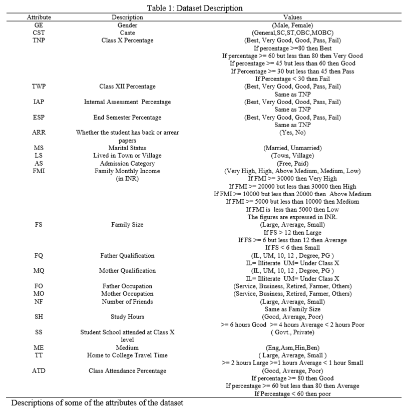
The purpose behind this project was to study data published by Hussain S, Dahan N.A, Ba-Alwi F.M, and Ribata N. in a paper titled “Educational Data Mining and Analysis of Student’s Academic Performance Using WEKA”. In this paper, the authors take data compiled regarding Indian school students and attempt to determine likelyhood of success using a variety of machine learning techniques. This type of analysis can be very important in determining what factors need to be addressed to improve student performance in school systems and prevent drop outs. It also opens a window allowing us to see into what kind of soceital issues play a part in academic performance.

In the paper the authors compare several types of algorithms such as Neural Networks, SVM, K nearest neighbors, and Random forest. These are used in classification tasks to determine whether a student will perform well, poorly, etc. Before running these algorithms, the authors use feature selection techniques to determine which features play the largest roles in the labels. Metrics used to evaluate performance were Recall, Precision, F-scores, MSE, MAE, and accuracy.

The label in this study is ESP, end of semester percentage. The dataset used for this study is freely available at UCI Machine Learning Repository. The authors were able to narrow down the feature dimensions to 15, using a variety of feature reduction methods.

This project will attempt to recreate the results systematically while learning about the effect of feature dimensions on outcomes. First, I will look at using all feature dimensions to predict outcome using KNN then with SVM. Then, I will narrow features to find the most important ones, and finally will compare the accuracy of the algorithms to determine which is most effective.

Predictions using all given features

Reading in the Data

The data will be read in using pandas with the following code:

 
    import pandas as pd
        performance_data = pd.read_csv('C:/Users/Aaron/Desktop/Python Files/academic_performance.txt', 
                               names=['Gender','Caste','Class_X','Class_XII',
                               'Int_Asses_Per','End_Sem_Per','Arrears','Marital','Town_City',
                               'Admission','Family_Income','Family_Size','Father_Edu','Mother_Edu',
                               'Father_Occ','Mother_Occ','Friends','Study_Hours',
                               'School_Type','Language','Travel_Time','Attendence'])

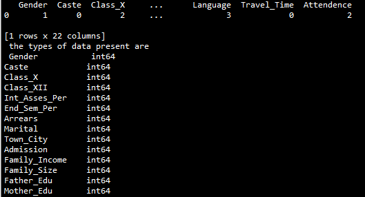
    print(performance_data.head(1), '\n the types of data present are \n', performance_data.dtypes)

From this we can see that all of our data types are of type “object”, which means we will need to map this to numeric values before using the data. To do this we will write a function that maps non-numeric values to numeric ones:

 
    import numpy as np
    def dataframe_converter(data):
      #first will create all of the column names in a array
      column_names = data.columns.values
      #now will loop over each column
         for column in column_names:
           value_dic = {}
           if data[column].dtype != np.int64 and data[column].dtype != np.float64:
            #now if a column isnt ints or floats we look into it
            #want to find all unique values in the column
            all_vals = data[column].values.tolist()
            #now find all the unique values
            uniques = set(all_vals)
            #now a value to map to 
            val = 0
            for unique in uniques:
              if unique not in value_dic:
                value_dic[unique] = val
                val +=1 
          #now map unique values to data
          data[column] = data[column].map(lambda x: value_dic.get(x))
        return data

and now can take a look at the data after its passed through.

We can see that the data types are now all int64. Perfect! We can run a quick check for missing or NaN values using ‘'’performance_data.isnull().values.any()’’’, but see that none are present. This is expected, as the data shown on the UCI website is complete. The metric I will attempt to predict will be end of semester percentage, like the paper evaluates. Separating into features and labels can be done using a simple df.drop command. Additionally, outliers will not be a problem since all possible values are categorical. Data preprocessing is taken care of using the scale function from scikit learn. So now we are done with data cleaning and are ready to move on.

A Niave Approach

As mentioned before, first we will run the complete data set through 3 algorithms and see how they perform before optimizing the data set to remove unnecesary features. The data will be split into training and test sets using cross_validation’s train_test_split. Now, I will compare the results of the KNN (K=6 because we have 5 classes available) and SVM. First, I’ll use KNN. Accuracy comes out to be $59.18\%$ (yikes). Below are pie charts of both the predictions on the test set, and the actual test set.

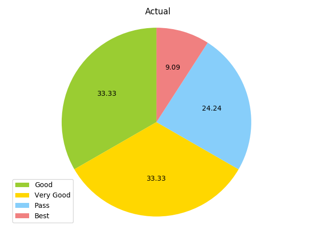
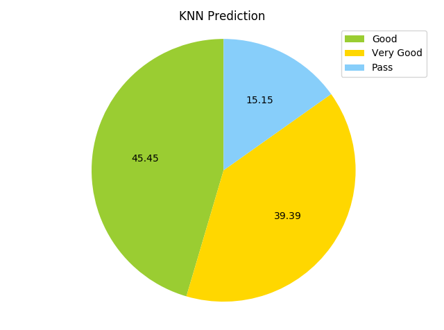
The KNN predicted no best scores, and was slightly inaccurate at best on other categories. Hopefully the SVM will do a bit better.

Running the SVM from scikit learn, I get an accuracy of $36.6\%$…really bad. The chart is shown below.

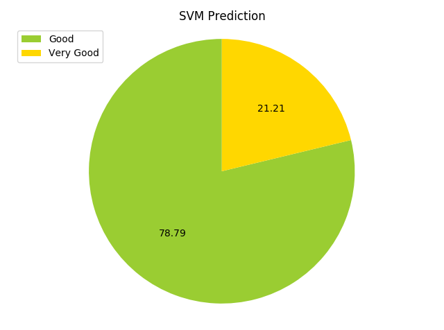
It’s obvious that the features need to be narrowed down. The shape of the dataframe is 131 rows and 22 columns, so the number of rows is not too much higher than the number of columns.

Dimensional Reduction

Univariate Selection

To reduce the dimensionality of the dataset to its most important factors, I will use a couple of different forms of dimensional reduction and see which one provides the best accuracy. The first method I will use is the SelectKBest method in Python. In this method, python can use a variety of statistical tests to find the best features. In this case, I will use the $\chi^2$ test. In this test, we reject or confirm a null hypothesis based on the sum of the squared errors divided by their expected value. If this sum when charted with a critical value called alpha is greater than the critical value, we can reject the null hypothesis. The code to find the new features is:

     
    from sklearn.feature_selection import SelectKBest
    from sklearn.feature_selection import chi2

    test = SelectKBest(score_func=chi2, k=9)
    fit = test.fit(x_train, x_test)

    features_reduced = fit.transform(features)
    #print('new reduced featureset shape is', features_reduced.shape)

    #now will find which ones are best
    feature_names = list(features.columns.values)

    mask = test.get_support() #booleans of the original set
    new_names = [] #list for new best features

    for bool, feature in zip(mask, feature_names):
      if bool:
        new_names.append(feature)
    print('The features found to be most important are:',new_names)

Using this procedure, I find that the optimal number of features is 9, and the most important features are the internal assesment percentage IAP (part of a continuous semester evaluation), arrears ARR (whether the student had failed any papers in the past semester), LS (whether the student lived in the city or country), admission category AS (whether the student had a free or paid tuition), the educational level of the father FQ, the occupation of the father FO, the number of friends NF, the native language ME, and the attendence percentage ATD. The factors line up with the factors found by the author, however, the author found 15 important categories whereas I find the optimal number to be 9. The 9 found in my optimization are a subset of the set found in the paper.

Decision Trees

Next I will use a bagged decision tree method, ExtraTreesClassifier, to determine feature importance. In this method we will use a series of decision trees to give a importance score to each attribute. First I will unpack and apply the sorting model

 
    from sklearn.ensemble import ExtraTreesClassifier
    #extract the features
    model = ExtraTreesClassifier()
    model.fit(x_train, x_test)
    print('for the extra trees the importance scores are', model.feature_importances_)

The authors proceed by finding the 15 most important attributes, so now I will make a dictionary of the 15 most important according to the ExtraTrees model.

 
    #create dictionary to map and rank features
    feature_importance_dic = {}
    values = (model.feature_importances_)

    for i in range(len(feature_names)):

  
    sorted_by_value = sorted(feature_importance_dic.items(), key=lambda kv: kv[1])

    print('from feature extra trees the 15 most important values are:', sorted_by_value[-15:])

Next, I will compare my 15 most important features to the ones found by the author. I will do this by repeating the following code for each possible feature reduction method used by the author

 
      my_list_trees = sorted_by_value[-15:]

      #get just the string labels from 15 most important
      my_list_trees_names = []
      for i in range(len(my_list_trees)):
        my_list_trees_names.append(my_list_trees[i][0])
      my_list_trees_names = sorted(my_list_trees_names)

      for i in range(len(my_list_trees_names)):
        if my_list_trees_names[i] == correlation[i]:
          corr_vals.append(1)
      corr_percentage = (len(corr_vals)/len(my_list_trees_names))

In the above code, I have sorted the 15 most important elements by value. The list my_list_trees includes names of features as well as their score, so next I remove the scores to leave me with a list of only the 15 most important names. Then I go about appending an empty list with an irrelevant value for each match with the author’s list. Finally, I divide the length of the matches list by the total length of the original list.

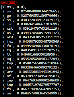
After comparing accuracies, I get that the list of important attributes that I find is a $100\%$ match with the author’s symmetrical uncertainty attribute selection method. The sorted list of least to most important features I find is

Try Optimized Features on the SVM and KNN

To use the optimized parameters on the classifiers, I need to select the most useful parameters from the full dataframe. This can be done using the following code:

 
    #need to select most important features
    optimized_features = {}
    feature2_names = (features2.columns.values)

    for i in range(len(my_list_trees_names)):
      for j in range(len(feature2_names)):
        if my_list_trees_names[i]==feature2_names[j]:
          optimized_features[my_list_trees_names[i]] = features2[feature2_names[j]]

In this code, after reloading the dataframe I create an empty dictionary which will be used to store the optimized dataframe, and create a list of all possible features in feature2_names. The optimized headers are stored in my_list_trees_names. Then, looping over each optimized header value, I look for a matching header in the feature2_names set. If a match is found, that column is added to the optimized features set.

After getting the new optimized dataset, a cross validation is performed as before and then the KNN and SVM classifiers are revisited. The accuracy of the KNN actually decreases to $\approx 57\%$. The SVM, however, increases accuracy from $36.6\%$ to $60.60\%$. A nice increase. Accuracy achieved by the BayesNet classifier in the original paper is $65.33\%$. The highest accuracy achieved in the paper is with the Random Forrests classifier. So lastly, to attempt to recreate the result, I will run the optimized features through this algorithm.

Putting the data through the scikit learn RandomForestClassifier is straightfoward, and gives an accuracy of $\approx 60\%$. The paper the data is based off of uses WEKA and does not provide optimization parameters for this project. So, in order to improve algorithm accuracy, I will attempt to hypertune parameters using RandomSearchCV. This uses a number of cross validation folds along with a number of iterations to randomly sample a grid of preset values in order to find the most accurate combination of parameters.

 
    for i in range(len(my_list_trees_names)):
      for j in range(len(feature2_names)):
        if my_list_trees_names[i]==feature2_names[j]:
          optimized_features[my_list_trees_names[i]] = features2[feature2_names[j]]
          # Number of trees in random forest
    n_estimators = [int(x) for x in np.linspace(start = 300, stop = 500, num = 5)]
    # Number of features to consider at every split
    max_features = ['auto', 'sqrt']
    # Maximum number of levels in tree
    max_depth = [int(x) for x in np.linspace(10, 110, num = 5)]
    max_depth.append(None)
    # Minimum number of samples required to split a node
    min_samples_split = [2, 5, 10]
    # Minimum number of samples required at each leaf node
    min_samples_leaf = [2, 4]
    # Method of selecting samples for training each tree
    bootstrap = [True]
    
    # Create the random grid
    random_grid = {'n_estimators': n_estimators,
               'max_features': max_features,
               'max_depth': max_depth,
               'min_samples_split': min_samples_split,
               'min_samples_leaf': min_samples_leaf,
               'bootstrap': bootstrap}
    pprint(random_grid)

    #Use the random grid to search for best hyperparameters
    #First create the base model to tune
    rf = RandomForestClassifier()
    # Random search of parameters, using 3 fold cross validation, 
    # search across 100 different combinations, and use all available cores
    rf_random = RandomizedSearchCV(estimator = rf, param_distributions = random_grid, n_iter = 100, cv = 3, verbose=2, random_state=42, n_jobs = -1)
    # Fit the random search model
    rf_random.fit(x_train, x_test)

After this tuning is complete, the optimized parameters can be used to refit the RandomForestClassifier. Once this is complete, the classifier gives an accuracy of $73\%$. Nice improvement! A visualization of a tree is shown below:

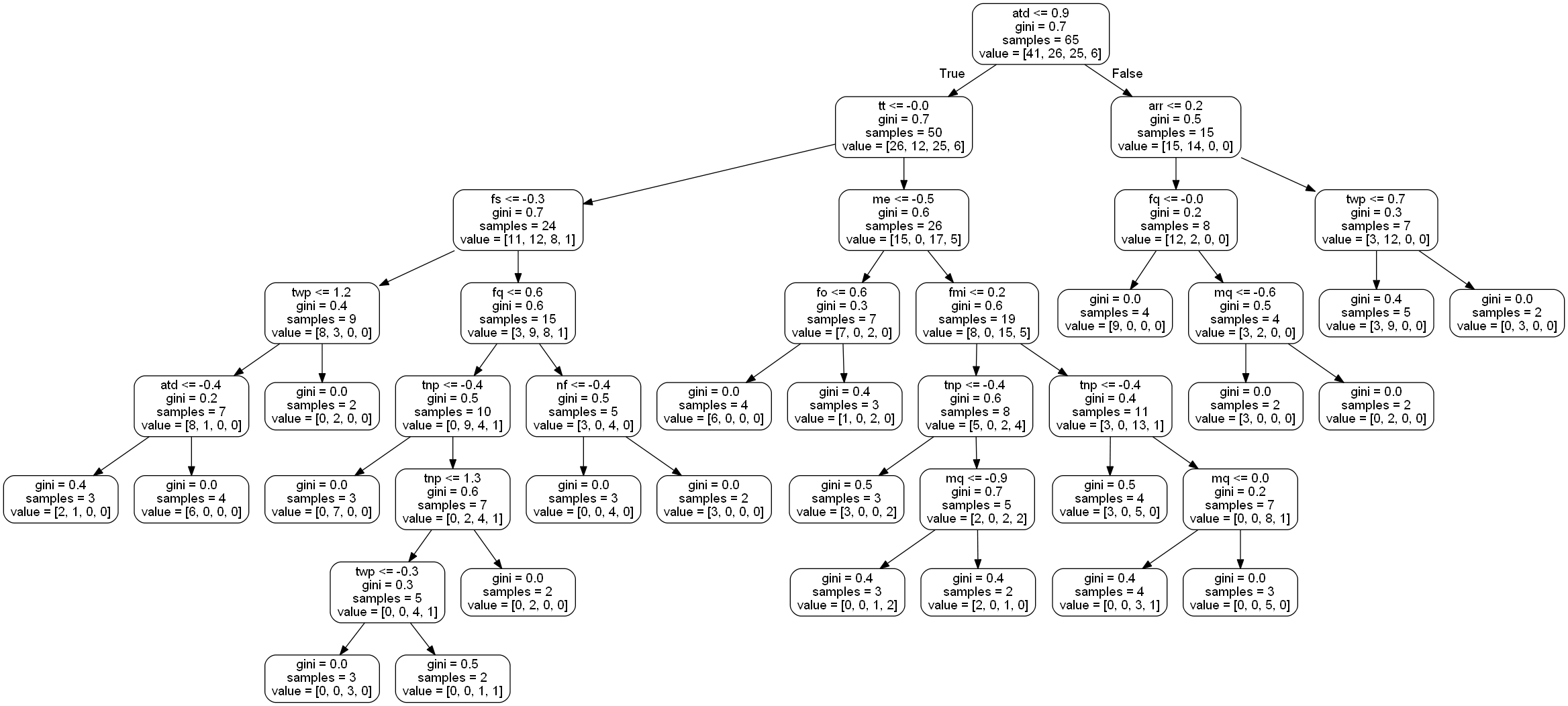
In order to increase this, we could increase the number of features available, or continue hypertuning using GridSearchCV to narrow in on the higher scores. Unfortunately, my little laptop cannot perform calculations beyond the one shown above. Although the $99\%$ goal was not reached, a nice increase from $50\%$ to $73\%$ can be seen. A large difference is made by optimizing feature dimensions and by hypertuning the classifier.

Data Visualization

Lastly, some nice conclusions can be drawn from looking at the most important features. I will choose 4 particularly interesting features to look at: the number of study hours (sh), the number of friends in the classroom (nf), the size of their family (fs), and the medium (me) which is their native language.

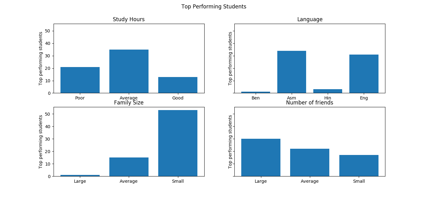
We can see from the uppermost left plot that the number of hours studied had a somewhat unexpected effect; it seems that there are diminishing returns for study hours. The number of students with a small number of study hours in the top performing bracket is small as expected, but the number of top performing students with an average amount of study hours is larger than the other two groups. Perhaps this is because the students with a large number of study hours were simply cramming for exams, whereas those with an average amount paid closer attention throughout the semester and didn’t need to prepare as long for the exam.

The family size plays a factor as well; within the top performing students, those with small family sizes formed the largest population. An explanation for this could be that those that came from small families had more attention paid to them individually by parents and family resources, vice a larger family where resources would have to be distributed more thinly.

Lastly, within the top performing students, those with the largest amount of friends had the largest represetation. This could be that having more friends in the classroom allowed for more idea sharing and collaborative learning efforts.

From this, we can see that encouraging group collaboration and distributed note taking could be ways to increase overall student performance in the classroom.