Regression from Scratch

Project Objective

The purpose behind this project was to dig into the mathematics behind a typical regression algorithm. Once the mathematics were fully grasped, the next step was to write from scratch an original regression algorithm. Finally, the comparison would be made between my personal algorithm and the scikit learn algorithm in Python.

The Theory Behind Linear Regression

Imagining a simple problem in which we have input data $x\in \mathbb{R}^1$ and a scalar label set $y\in\mathbb{R}^1$, a plot might look like (data generated using x, y = make_regression(n_samples=100, n_features=1, noise=10))

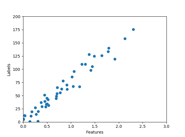
In such a plot, it is quite easy to see that the brunt of the data falls along a line which might be described using a simple funcion such as $y=mx+b$. In the arena of data science, we would refer to the variables in this equation as $w_0$ and $w_1$, also known as the bias and slope. The goal in a linear regression calculation would be to find a function, $\mathcal{f}(x)$, which maps the domain data, $x$, to the output data, $y$. This function is called the regression function and has two parameters (for the case of 1D data) to be determined, namely, the slope and bias.

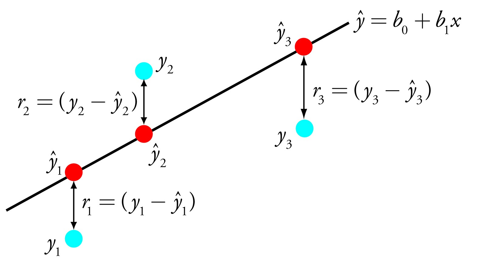
For input data generalized to $d$ dimensional data, the equation to solve becomes $y_i \approx \mathcal{f}(x_i) = w_0 + \sum_{j=1}^{d}x_{ij}w_j$. The problem is now set up. The next step to take is to find an objective function which provides us with satisfactory values of the slope and bias. The function we will use for this is the least squares function:

$$w = argmin \sum_{i=1}^{n}(y_i-\mathcal{f}(x_i))^2$$

What we are doing is summing over each data point and at each data point finding the difference between the actual truth value and the value predicted by our regression function. Minimizing this error will give us satisfactory values for the hidden variables $w_0$ and the slope.

The formula above holds, however can be simplified using vector notation along with linear algebra. Before beginning, we will extend the input data by one dimension to take account of the bias. We can write a $d$ dimensional data point as

$$x^T = \begin{bmatrix} 1,&x_{i1},&x_{i2},&...&x_{id}\\ \end{bmatrix}$$

Because each of these dimensions will have their own slope, we can also write a vector of $w$’s as

$$w = \begin{bmatrix} w_0,&w_{1},&w_{2},&...&w_{d}\\ \end{bmatrix}$$

We now want to find the maximum likelyhood of the least squares function with respect to vector $w$. This can be done using the gradient (for n data points)

$$\sum_{i}^{n}\nabla_w(y_i^2-2w^Tx_iy_i + w^Tx_ix_i^Tw) = 0$$

which can be solved to give

$$w_{LS} = (\sum_{i=1}^{n}x_ix_i^T)^{-1}(\sum_{i=1}^{n}y_ix_i)$$

And easy extension of this notation is moving into matrix form. Following the exact same procedure, we can derive the result

$$w_{LS} = (X^TX)^{-1}(X^Ty)$$

Where $y$ is now a vector, and $X$ is a matrix of dimension $n\times(d+1)$. New data can then easily be found using the relation $y_{pred} \approx x_{new}^Tw_{LS}$

This method is nice and self contained. However, there are limitations. As we can see from looking at the final (matrix) form of the solution for $w_{LS}$, the matrix $(X^TX)$ must be invertible. Equivalently, the matrix must be full rank. This means that all rows and or columns must be linearly independent (cannot be tranformed into one another using multiplicative constants). If we were to write this matrix in row reduced echelon form, all pivot positions would be occupied by 1’s. If $(X^TX)^{-1}$ does not exist, then there are infinite possible solutions. To prevent this, we want $n\gg d$, or the number of data points to outnumber the dimensions of our data. This is a real consequence of the curse of dimensionality.

Lastly, before moving on to actually code this, we need to extend the problem a bit. Simple linear regression only works for a subset of all possible data we can come across. In reality, data can take many different forms in which a linear fit might be better approximated by a higher order polynomial fit. In this case, we can extend the equations as follows

$$y = w_0 + w_1x + w_2x^2 + w_3x^3 +...$$

This is still, however, linear regression, because we are still linear in the unknown parameters $w$. The matrix we are working with then becomes (for 1 dimensional data and a $p^{th}$ degree polynomial):

$$X = \begin{bmatrix} 1,&x_{1},&x_{1}^2,&...&x_{1}^p\\ 1,&x_{2},&x_{2}^2,&...&x_{2}^p\\ \vdots&& &...&\vdots \\ 1,&x_{1},&x_{1}^2,&...&x_{1}^p\\ \end{bmatrix}$$

which means we can solve exactly as before. Finally! We’re ready to start coding.

Writing a Regression Script

For this script, I will be using python. I will be writing this function using 1 dimensional data taken from the classic boston housing dataset. An obvious extension of this program would be to include data of any dimension. However, the purpose of this was to understand the inner workings of the regression algorithm. To actually use this script on a dataset inplace of a (for example) scikit learn fit would require some additional effort. Lastly, this is run as a script. To call this in different examples it would be best to use object oriented programming and create a class. Leaving it in the script format, though, makes it easier to tinker with. First I will import the necessary packages and dataset

 
    import numpy as np
    import pandas as pd
    import matplotlib.pyplot as plt
    from sklearn.linear_model import LinearRegression 
    from sklearn.model_selection import train_test_split 
    from sklearn.preprocessing import PolynomialFeatures
    from sklearn.pipeline import make_pipeline


    #get some test 1D data
    file_path = 'C:/Users/Aaron/Documents/boston_data.xlsx'
    boston_data = pd.read_excel(file_path)


    #input data as a list, already gives x_n
    features_in = np.asarray([boston_data['CRIM']])
    #input labels as a list as well
    labels_in = np.asarray([boston_data['MEDV']])
    row, cols = features_in.shape

Then, as discussed above, the dataset will need an extra dimension added to it of value 1. Also the polynomial degree will be included at this point. Polynomial degree can be seen in the dimensions of the $X$ matrix

 
    #create big matrix X composed of each row as a data point, up to degree of polynomial
    #take degree of polynomial
    p=2
    #want to add a dimension to x of 1 to p to account for offest
    X = np.zeros(shape = (cols,(p+1)))

    #first add one to the first column of X
    for i in range(cols):
    X[i,0] = 1

    k=0

    for i in range(cols):
        for j in range(1,p+1):
            X[i,j] = features_in[0,i]**j

Now I will make use of the formula $w_{LS} = (X^TX)^{-1}(X^Ty)$, and calcuate the transpose of the $X$ matrix

 
    X_t = np.transpose(X)
    X_tX = X_t@X
    w_ls = (np.linalg.inv(X_tX))@(X_t@np.transpose(labels_in))

After calculating the optimized least squares, I will look at a scatter plot of the actual features and labels overlaid with the predicted points from the regression, and calculate the mean square error of the prediction.

 
    plt.scatter(features_in,labels_in)
    plt.plot(np.transpose(features_in),X@w_ls,linestyle = '',marker='o',color='r',zorder=1)

    #find MSE
    print('the mean squared error of my model is',(np.mean((labels_in)-X@w_ls)**2))

The plot is shown below:

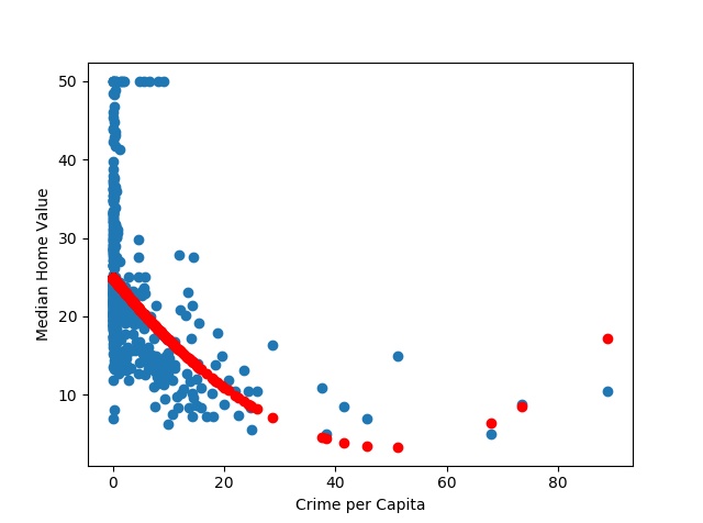
Th mean square error given is $357.939$. Now, the next thing to do is compare this with the scikit learn regression function. This can be done using the following code

    plt.scatter(features_in,labels_in)
    boston_dataframe = pd.DataFrame(boston_data)
    features_data = boston_dataframe['CRIM']
    features_data = features_data.values.reshape(len(features_data),1)


    labels_data = boston_dataframe['MEDV']
    x_train, y_train, x_test, y_test = train_test_split(features_data,labels_data)

    lm = LinearRegression()

    #now compare this to a polynomial fit
    p=make_pipeline(PolynomialFeatures(3),LinearRegression())
    p.fit(x_train,x_test)
    p_pred = p.predict(y_train)

    plt.figure(3)
    plt.scatter(features_in,labels_in)
    plt.plot(y_train,p_pred,linestyle='',marker='o',color='r')

In which $makepipline$ has been used to get a second degree polynomial fit, the same polynomial order used in the homemade fit. The scatterplot is shown below:

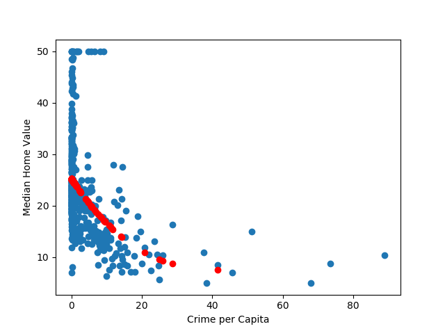
And the mean square error of this comes out to be $537.84$, pretty close to the homemade prediction! Further refining the homemade model to take into account regularization and other factors could further improve it.